How LLMs Answer

Part 2 of the deep-dive series, picking up from How LLMs Get Built. Part 1 covered the months-long pipeline that produces the model. This post is the other half: the millisecond pipeline that runs every time you hit Enter.

The Map closed Part I with the trained model: weights frozen, ready to serve. Part II starts when your prompt arrives.

Same weights, different code path. The artifact that took six months to build now has 200 milliseconds to respond before users notice the lag.

Training is one shape: read trillions of tokens, adjust weights, repeat. Inference is a different shape: read one prompt, generate one token at a time, never adjust anything. The model that answers your prompt is frozen. Every response uses identical weights. Only the input changes between requests.

Inference is also two programs, joined by a data structure that exists nowhere else in computing. That structure is the KV cache, and it’s why streaming generation is economically possible at all.

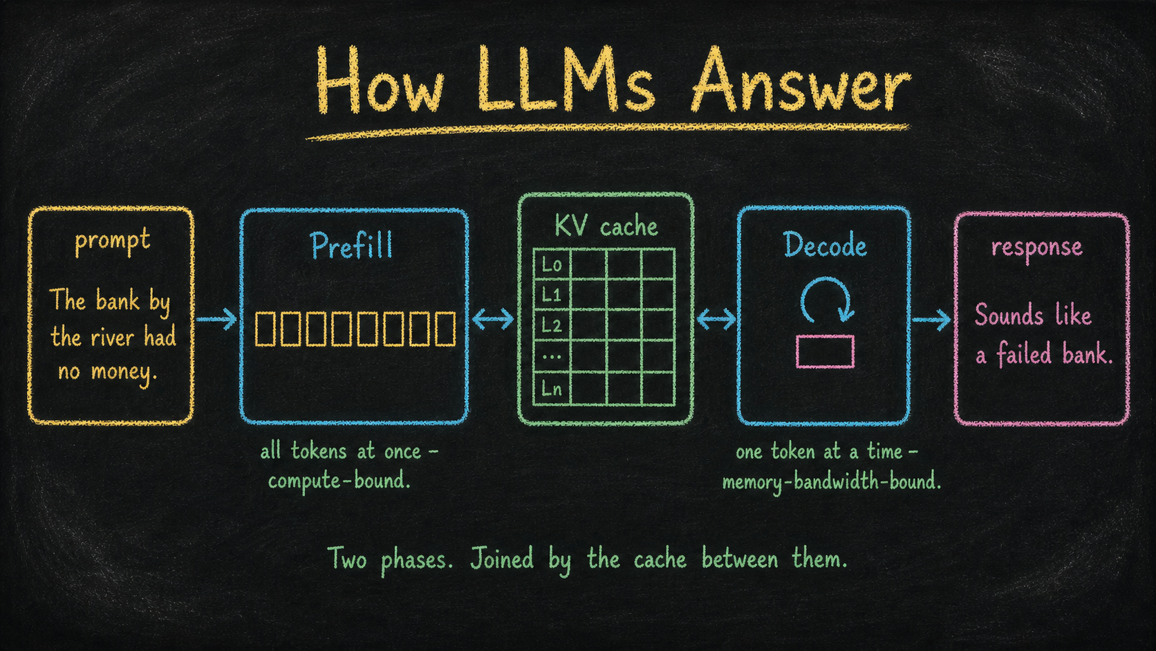
By the end of this post, the pipeline should sit in your head as a specific sequence: prompt assembly, prefill, decode, optional tool use or extended thinking, response. Five structural steps. Two distinct compute regimes. One cache between them.

1. The prompt is not your message

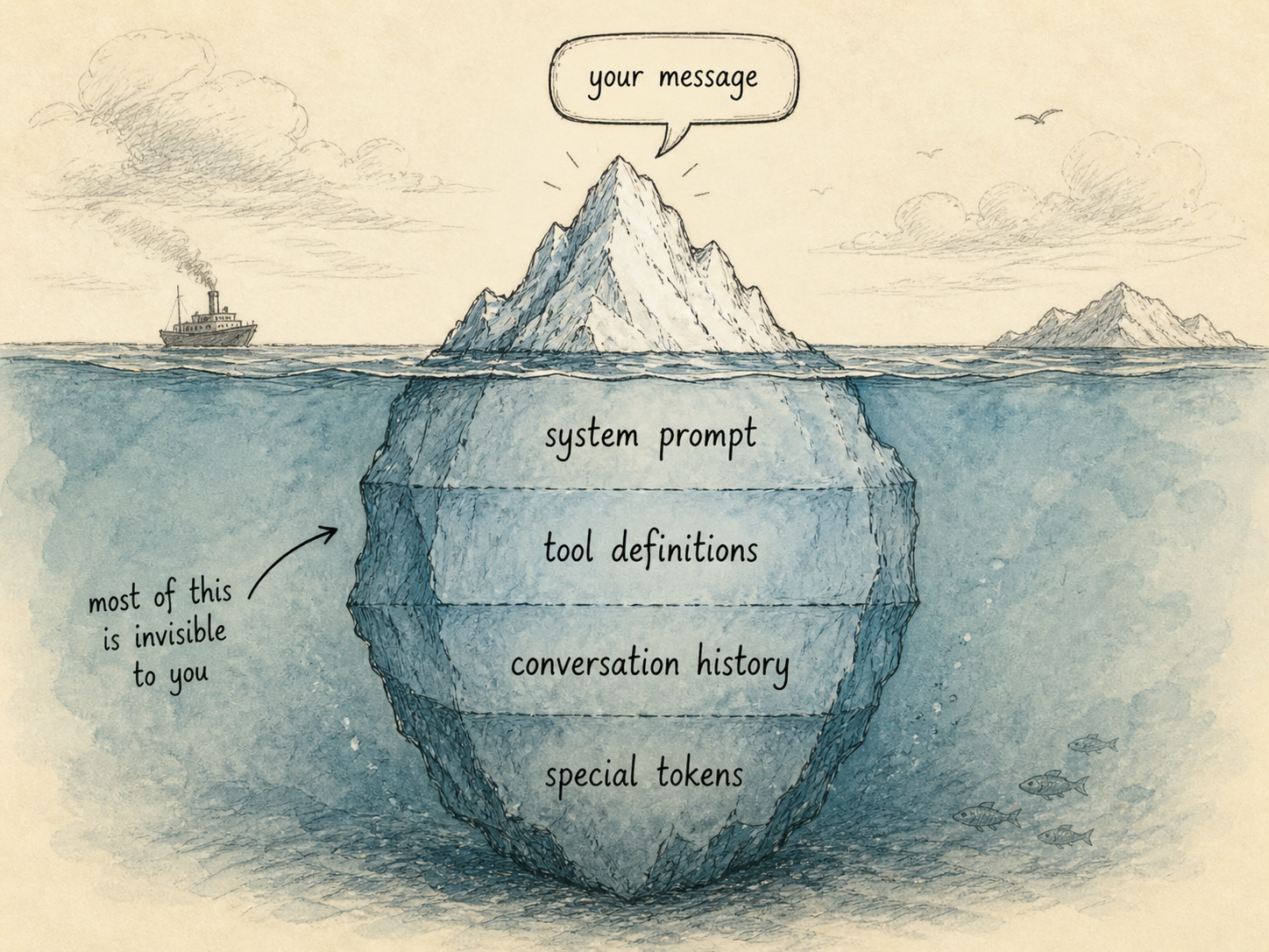
You typed one sentence. The model receives thousands of tokens.

Before any GPU work happens, the server assembles what’s actually going to be tokenized. Your message is the last piece, not the only piece:

• System prompt: safety instructions, behavioral guidelines, current date.
• Tool definitions: JSON schemas for every tool the model can call. In Claude Code, this includes Read, Edit, Bash, Grep, and dozens more.
• Conversation history: every previous turn, including the model’s prior responses.
• Special tokens: delimiters that mark where each role’s message starts and ends.
• Your message: the text you actually typed.

A typical Claude Code prompt is 5,000 to 50,000 tokens before you’ve said anything. This matters because every token in the assembled prompt has to be processed by the GPU before the model produces its first response token. Longer prompt, longer wait.

Routing happens in parallel. The same model name (Claude Opus 4.7, GPT-4o) maps to dozens of GPU instances around the world. The API gateway picks one based on geography, current load, and which instances have your conversation prefix already cached. If your previous turn ran on Instance 47 in Virginia and Instance 47 still has your KV cache in memory, you get sent back to Instance 47. This is invisible from the outside but has dramatic latency implications.

Authentication, rate limits, and quota checks happen before any of this. If your key is invalid, the request never touches a GPU.

2. Prefill: the prompt enters the GPU

The assembled prompt is tokenized using the same merge table that was frozen during training. This step runs on the CPU and is fast: millions of tokens per second. The output is an array of integers.

Then the array hits the GPU, and the first phase of inference begins.

Prefill is the model processing your entire prompt in one parallel pass. Every token gets embedded, every layer runs, every attention computation happens, all at once. This is what GPUs are designed for. Thousands of tokens, computed in parallel, in a few hundred milliseconds.

Make that concrete.

Take the running example from The Map: The bank by the river had no money. Eight tokens, processed in one parallel pass. The phrase had no money is the decisive constraint here. Financial banks can run out of money; riverbanks don’t have money in the first place. So even though “river” sits closer to “bank” in the sentence, “money” is the more informative signal for what “bank” means - and by the time prefill finishes, the cumulative representation has resolved “bank” to the financial-institution reading. The disambiguation happened in a single forward pass, no iteration needed.

The output of prefill is two things:

1. A logit vector for the last token, used to sample the first response token.
2. The KV cache: every key and value vector, at every layer, for every token in the prompt, stashed in GPU memory so it never has to be recomputed.

That second output is the interesting one. Without the KV cache, generating each new token would require re-running the entire prompt through the entire model. With the cache, only the new token has to flow through. This is the architectural detail that makes streaming generation economically viable.

Prefill is compute-bound. The GPU’s bottleneck is matrix multiplication throughput. Doubling the prompt length roughly doubles prefill time. This is why Time To First Token (TTFT) scales with prompt length: the longer your context, the longer you wait for the first character.

A 1,000-token prompt prefills in roughly 50ms on Anthropic-class infrastructure. A 100,000-token prompt prefills in roughly 5 seconds. The math is roughly linear.

3. Decode: the autoregressive loop

After prefill, the model has produced one token. To produce the second token, it has to feed that token back into itself.

The decode loop:

1. Take the most recently generated token.
2. Embed it. Run it through every transformer layer.
3. At each attention layer, compute Q, K, V for just this token. Read K, V from the cache for all previous tokens.
4. Append this token’s K, V to the cache.
5. Compute logits over the full vocabulary.
6. Sample one token from the distribution.
7. Convert the token ID back to text. Stream to the user.
8. Check stop conditions: EOS token, stop sequence, max tokens.
9. Repeat.

Take the running example forward. After prefill, the cache holds everything for The bank by the river had no money. Decode begins. The model samples a first token - “Sounds” - feeds it back as input, samples “like,” feeds it back, samples “a,” and on. Token by token, a response streams: Sounds like a failed bank. What didn’t happen: the model didn’t reply Sounds like a dry riverbank, because had no money had already pulled “bank” toward the financial reading during prefill. The response inherits the disambiguation.

Decode is memory-bandwidth-bound. Reading the model’s weights from GPU memory dominates the cost. The actual math (one token’s worth of multiplications) is trivial. What’s expensive is reading 30 to 200 GB of weights from HBM through the GPU’s memory bus, once per generated token.

This is why generation speed (tokens per second) is roughly constant regardless of prompt length. Whether your prompt was 100 tokens or 100,000, each new token requires the same memory traffic. A modern serving stack hits 50 to 200 tokens per second on a single GPU, depending on model size and quantization.

Sampling shapes the distribution before a token is chosen:

• Temperature rescales logits. Higher means flatter distribution and more randomness. Lower means peakier and more deterministic. Temperature 0 picks the top logit deterministically.
• Top-k keeps only the k most likely tokens, discarding the rest.
• Top-p (nucleus) keeps the smallest set of tokens whose cumulative probability exceeds p.

These knobs don’t change what the model knows. They only change how the next token is picked from the distribution the model already produced.

4. Tools and thinking: the agentic loop

Two extensions sit on top of the basic prefill-decode pipeline. Both run inside the same machinery; neither requires a different model.

Tool use is interrupted generation. The model is trained to emit a structured tool call when it needs to do something it can’t do internally. When that happens:

1. Generation stops. The response streams back with stop_reason: "tool_use".
2. The client (Claude Code, your application) executes the tool locally: reading a file, running a command, hitting an API.
3. The tool’s result becomes a new message in the conversation.
4. The server assembles a new prompt: original prefix + assistant’s tool call + tool result.
5. Prefill plus decode runs again on the new prompt.

Each tool call is a full round-trip. A single user message in Claude Code might trigger fifteen tool calls and fifteen prefill-decode cycles before the assistant’s final answer streams back. Without prompt caching, every cycle would re-process the entire previous context. With prompt caching, the unchanged prefix is recognized, its KV cache is retrieved from a cache pool, and only the new portion (the tool result plus a few tokens of tool-call markup) needs to be prefilled.

This is why prompt caching matters economically. A typical Claude Code session might process 200,000 tokens of cached context for every 5,000 tokens that are actually new. Cache writes cost slightly more than uncached input; cache hits cost a fraction. Over a long session the discount is roughly an order of magnitude.

Extended thinking is the same machinery applied to internal reasoning. When Claude uses extended thinking, it generates reasoning tokens into a thinking region before producing the visible response. There’s no separate “thinking module” in the architecture. The model just generates tokens that the API marks as thinking and the client doesn’t display. Those tokens still occupy context, still cost compute, still influence the final answer through attention.

This is why higher thinking budgets produce better answers on reasoning-heavy tasks. The model has more space to deliberate. The cost is more decode steps. Thinking tokens are real tokens, billed and rate-limited like any other.

5. Batching, caching, and the economics of serving

A single GPU running a single user’s request would lose money. Inference is economic only because of three optimizations stacked together.

Continuous batching. Many users’ requests run on the same GPU at the same time. The serving system (vLLM, TensorRT-LLM, SGLang) interleaves them: one user’s decode step runs while another user’s prefill is finishing. Each weight is read once and used to generate tokens for many users simultaneously. This is what makes the per-token economics work.

Paged attention. KV caches are large and have variable lengths. Naïve allocation wastes memory. Paged attention treats GPU memory like virtual memory: cache blocks are allocated in fixed-size pages, mapped through a page table. Fragmentation goes away, and the system packs more concurrent users onto each GPU.

Speculative decoding. A small “draft” model produces a few candidate tokens cheaply. The full model verifies them in parallel, accepting the draft (fast path) or rejecting and falling back to its own prediction (slow path). When the draft model is right, which it usually is for predictable text, decode runs 2 to 3 times faster.

The serving infrastructure also handles output moderation (a separate small classifier that checks the generated text for safety violations) and usage accounting (counting input tokens, output tokens, cache hits, cache writes, each priced separately).

When the final token streams to your terminal, the request closes, the KV cache is either evicted or kept warm for the next turn, and the GPU moves on to the next batch slot.

What’s Next

The inference pipeline is the same shape every time you hit Enter. Prefill processes the prompt. Decode generates the response. The KV cache is what lets the second phase exist at all. Tool use and extended thinking are extensions of the same loop, not different pipelines. Batching, caching, and speculative decoding turn unprofitable per-request math into a serviceable economy.

Most of inference isn’t neural-network code. The model itself is a stack of transformer layers, identical to what came out of training. Everything else (the gateway, the prompt assembly, the KV cache, the batching system, the cache management, the streaming protocol) is conventional engineering.

The intelligence lives in the weights. The economics live in the surrounding code.

The next post in the series goes inside one of those layers: attention specifically. What “bank” attending to “money” actually means at the level of matrix multiplications, why plausibility beats proximity in disambiguation, why multi-head matters, and what FlashAttention changed in 2022 that made all of this run on the hardware you can actually buy.

---

References

• Kwon et al., “Efficient Memory Management for Large Language Model Serving with PagedAttention” - vLLM, paged attention (2023)
• Dao et al., “FlashAttention” - IO-aware attention (2022)
• Leviathan et al., “Fast Inference from Transformers via Speculative Decoding” - Speculative decoding (2023)
• Pope et al., “Efficiently Scaling Transformer Inference” - PaLM inference, prefill vs decode breakdown (2022)
• Anthropic, Prompt Caching documentation - Cache control API
• Anthropic, Extended Thinking documentation - Reasoning tokens API
• Anthropic, Tool Use documentation - Tool calling
• vLLM, project page - Reference open-source inference server